Introduction
Final project for CS384G Spring 2016 at the University of Texas at Austin
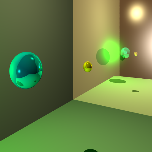
One of the problems faced in traditional ray tracing is global illumination. Though a certain degree of global illumination can be acheived in the traditional method (for instance, reflection, refraction, shadows), other effects such as caustics and diffuse-color-bleeding are not. Photon Mapping, a technique developed by Henrik Wann Jensen, resolves these issues. Whereas traditional ray tracing only accounts for the observer's perspective in the shading model, photon mapping incorporates both the observer's and the lights' perspectives. As such, effects that are easy to compute from the perspective of the light, such as caustics, and effects that are easy to compute from the user's perspective, such as specular reflections, and refractions, are all incorporated in the photon mapping shading model.
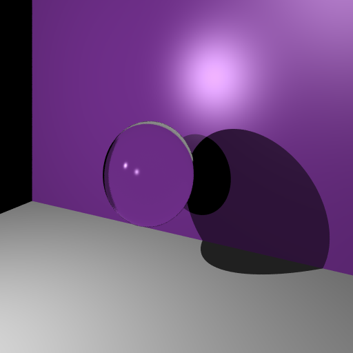
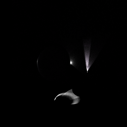
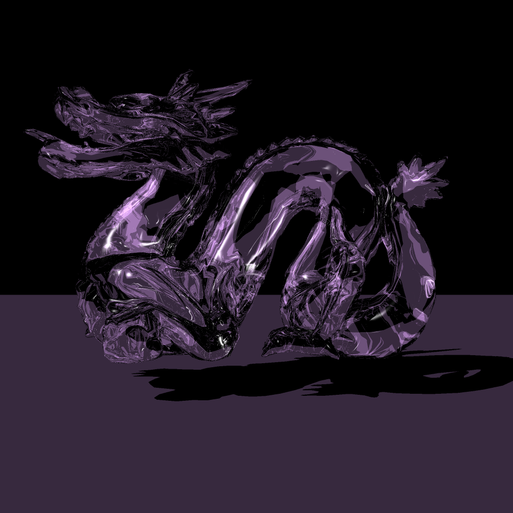
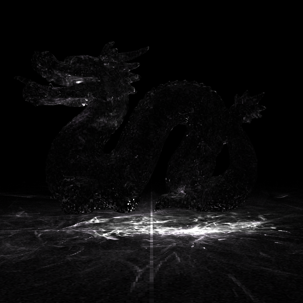
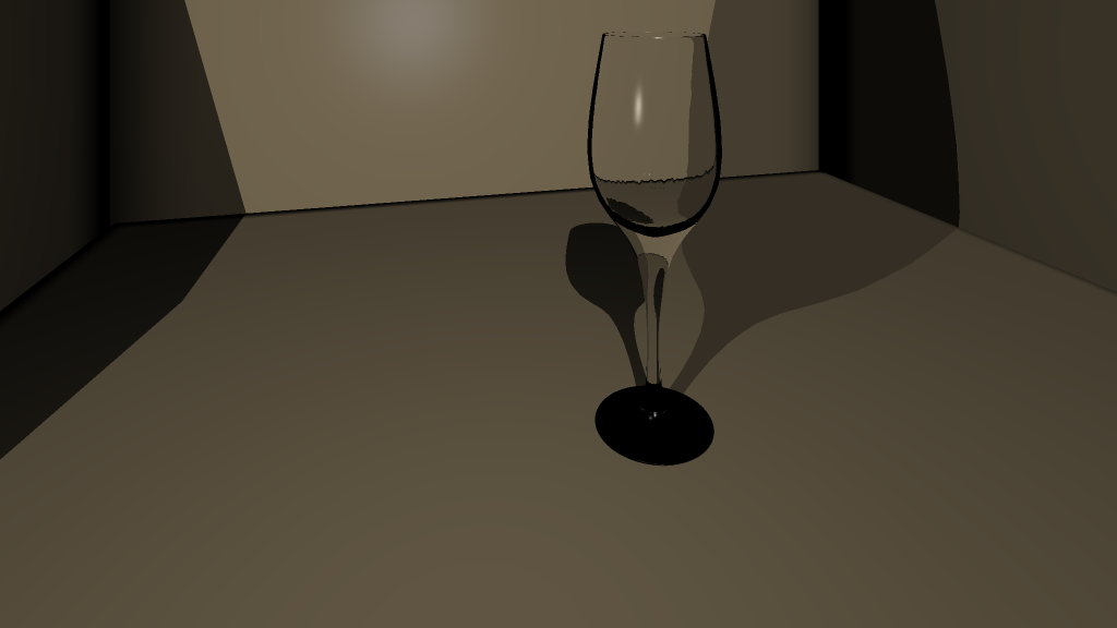
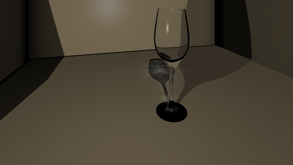
In this blog post, we outline a basic overview of Photon Mapping, and present our implementation of it, along with a discussion of how our implementation differs from that in most literature. We also include some of the output images from our algorithm, separated out into three buffers: the first depicting the original (ray-traced) rendered, the second with the photon map, and the third depicting a screen overlay blending of the first two buffers.
Photon Mapping Basics
Photon mapping is achieved via a two pass algorithm. The first stage actually computes the photon map by firing photons from each light source into the scene in much the same way as traditional ray tracing fires rays from the camera into the scene. The photons are stored in some data structure for later aggregation. Effectively, the second pass is a traditional ray tracer where the shading model incorporates cumulative photon intensities in some local neighborhood.
In Jensen's original photon mapping method, the photons are stored in a balanced axis aligned KD-tree and keep track of photon intensity, intersection positions, angle of incidence, and other metadata for future aggregation. During the second pass of the algorithm, when a ray intersects an object all photons in a local sphere are aggregated and the radius of the sphere increases until a predefined energy condition is met. Consequently, total number of photons launched into the scene, photon intensities, minimum sphere radius, maximum sphere radius, and minimum total energy are all hyper-parameters to tune.
Our Architecture
Rather than computing aggregating the photons in the second pass, we opt to aggregate them in the first pass using a spatial hash. By predefining a bucket size (or sphere radius), we can trade spatial precision and accuracy for speed. In fact, this method achieves O(1) photon map access time. Furthermore, we no longer have to worry about the near neighbor search since this information is encoded directly into the data structure. In the second pass, we compute the raytraced image and photon map image simultaneously, but save their values into different buffers. Since we use a spatial hash, our photon map image is rather speckled, so we apply a gaussian blur before screen blending it with the raytraced image.
Creation of Spatial Hash (Pre - Raytracing)
firePhotons():
    For each light source:
        emit n photons towards the bounding boxes of each object (this step can be parallelized)
        tracePhoton(depth)

tracePhoton(depth):
    if (photon intersects scene object AND object is closest object):
        if surface not reflective and not refractive:
            absorb photon (see 3)
        if surface reflective:
            if absorbPhoton( 1 - kr ):
                return
            else if not absorbed:
                reflect photon
                tracePhoton(depth-1)
        if surface is transmissive:
            if absorbPhoton( 1 - kt ):
                return
            else f not absorbed:
                refract photon
                tracePhoton(depth-1)

//(The above method uses Russian Roulette. Since no new photon is created, energy is conserved.)
// Absorb photon with probability p
absorbPhoton(p):
    if(rand() < p):
        photonMap[IntersectionPoint] += photon
        return true
    else:
        return false
By this point, we have the flux at each position of the spatial hash.
Creation of the Photon Buffer (During Raytracing)
PhotonColor = alpha * ImageColor + (1 - alpha) * photonMap[IntersectionPoint].flux
Ray Tracer Features
- Path Tracing / distribution ray tracing
- Jittered sampling
- Up to 16x super sampling
- Templated KD-tree acceleration using SAH
- Interpolated textures
- Cube Maps
- OBJ loading
- Photon Mapping
- Configurable number of photons and photon energy
- Point lights and Directional lights fully supported
- Note: Photons only fired towards extents of objects.
- Basic Image enhancement API (Gaussian kernels, Sobel operators, mean filters, etc)
Pretty Pictures
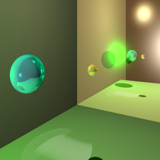
Color Bleeding Example
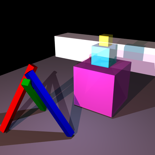
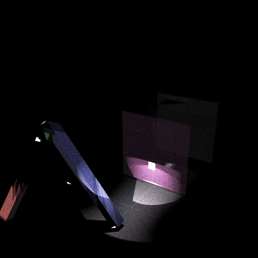
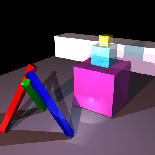
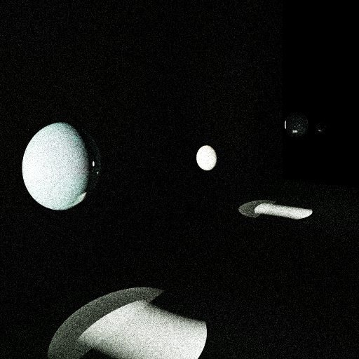
Caustics Example

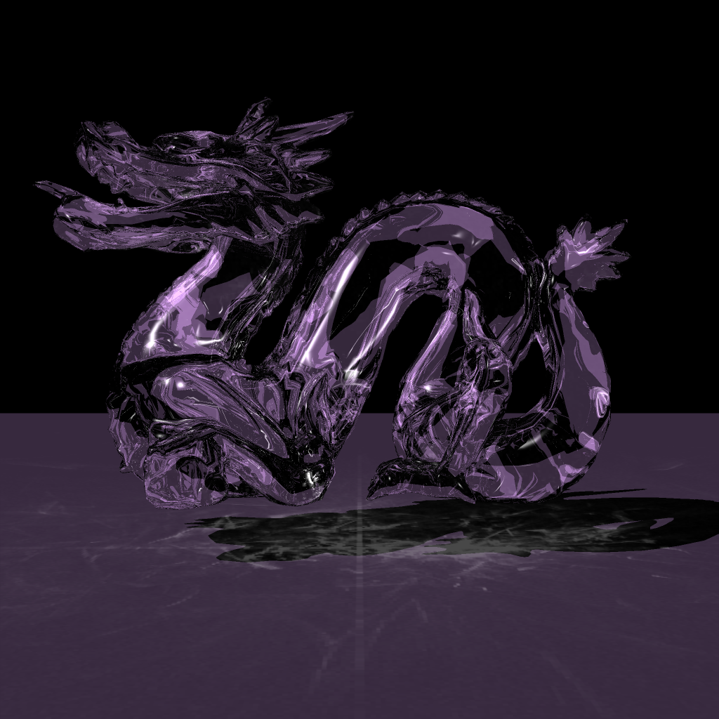
Other Cool Examples
Authors and Contributors
Michael Bartling (@mbartling), Souparna Purohit (@limac246)